Welcome back everyone, for at long last, the last in this vector series. It’s been a long haul, and I appreciate everyone who has come along for the journey.
In light of the happenings recently in the United States of America, I’d just like everyone to take a moment of silence; for those victims of prejudice, hate, and discrimination. Humans are social creatures, and we all need to realize we are here not in-spite of each other, we are here because of each other. It is our duty, no matter your role in society, your job, your socioeconomic standing, to treat all other individuals with the same standard of decency, respect, and humility. We all face challenges, some more than others, and as humans we must empathize with our fellow human, regardless of ethnicity, gender, or sexual preference. It is our unique ability as humans to be self-aware, we should use this power for good, and not evil. I challenge you to pause for a moment and imagine what it would be like to live in someone else’s shoes, someone who has to deal daily with prejudice and segregation; if only for a moment. I have been blessed with many opportunities in my life, and am thankful everyday for that. No matter our position in life, it is never our right to deny others a chance at the opportunities we have had. In fact, it is our responsibility, to help enable those opportunities for others. We mustn’t allow this to continue. After the protests have dispersed, and the smoke has settled. We must remember this, and as a society we must change. For if nothing changes, nothing changes. #blacklivesmatter
Thank you.
The last time we left of, we had a pretty much working vector implementation. Then we wanted to enable it to be used with standard algorithms. it was a bit of a trick though, because it already worked with the algorithms, using a direct pointer into the memory. Instead we wrote an iterator class that was a bit safer, and allowed us a bit more control over the raw pointer. Then we learned a bit of funny business with SFINAE, to enable specific functions only when the arguments are iterators. It was a pleasant stride that we took, and we learned a few things along the way. Taking a look at insert allowed us to meander down the valley of memory allocation, and reorganization. Then we were able to stop and smell the SFINAE roses, though they often have an off scent. At the start of this journey, I’ll be honest — I wasn’t expecting it would be this much work. It is crazy to think about the amount of brain power that went into crafting our humble little standard vector, that we use daily. It puts in perspective the amount of work that goes into the STL alone. Although, it was the premise of this series to illustrate why it’s in our best interest to use the fantastic set of tools that ship with our compiler.
This adventure however, is coming to a conclusion. When I started, I had almost jokingly said I wanted to pit the vector we would create, against the MSVC standard vector. At that time of writing, I didn’t really know what I was going to do, (similarly with “use it with the algorithms”). It isn’t to say I didn’t have a direction, I just didn’t know what I was going to do. So I had to decide what exactly “pitting my vector” against Microsoft’s meant. Luckily, since it’s my blog, it’s my arena. Though if I didn’t do it justice, I knew that I would get down-voted into oblivion. LIKE THAT TIME I THOUGHT VIM COULDN’T NAVIGATE TO HEADER FILES. So, I had to actually put some brain power into this, other than just making some asinine competition up, and declaring that I win!
We really want to measure the amount of work the vector is doing. Often in computing the amount of work is measured by the amount of processing time. This is why we say an operation, or algorithm is fast or slow, it’s the amount of time it takes to complete. It follows, that the less a particular operation does, the faster it will be. The fastest program, is no program at all. However, it’s also the most useless program ever. The art of optimization, is to do less work while still having the same outcome. There are a few things that affect the actual timing of operations. These things range from processor speed, program load (i.e. how many programs are running simultaneously), memory consumption, etc. These though, are all environmental. Meaning that if you tested program A, in the same environment as B, they should have the same effect. The biggest affect on your operations overall speed, will be it’s algorithmic complexity. You might’ve heard of this, sometimes it’s called Big-O notation. That is a constant time operation. You’ll hear people say things like a binary search is Log(N), or that a linear search runs in linear time. Worst of all, an algorithm is exponential. Now, these “time” measurements, aren’t actual wall clock time. Though, they will affect the amount of ticks your algorithm takes to complete. They’re a relative time scale, based on the amount of work the algorithm has to do. If an algorithm is linear, it means that as the amount of work the algorithm must do grows, the time will grow linearly in relation to size of it’s input. When something is a constant time operation, it means that it has to do the same work, regardless of the size of input.
Let’s explain this in-terms of our vector; Let’s say we want to find an item in our vector. In the first case we want to find the 10th item. Okay, so regardless of ordering of our vector, if we want the 10th item, we have to do the same constant work. We need to get the start of the vector, increment it by 10, and we have the item. Okay, Okay. What about a vector of size < 10. So we have to check the size first. Regardless though of our vectors size, it’s the same work for 1, 10, 100, 1 000, 10 000, 1 000 000 000 items. This means it’s a constant time operation. You would see this in the wall clock time. If the operation took 10 ms for a vector of 10 items, it would take roughly the same 10 ms regardless of the size.
What if we wanted to find an item that matched some predicate? Assuming our vector is a vector<int> of random numbers, and we wanted to find say the value 10. What do we have to do? Well, we have to start at the beginning and iterate the vector, until we find the value 10. Now, all things being completely random, you may find the element right at the beginning, some where in the middle, or maybe it’s the very last element. Given one full iteration of the vector, you’ll be able to either a) find the element b) know it doesn’t exist. This is a linear, algorithm. The wall clock time, will grow roughly linearly as the size increases. Meaning that it should take roughly 10 times longer to find an element in a vector of 10 vs. a vector of 100, with a linear search. In practice however, if you measured this once, you might see something strange. Your vector of 10, might take more time than the vector of 100. Why is that? Well, it could simple be due to a roll of the dice. All things being random, you found the item at the end of the 10 item vector, and it was the first element in the 100 element vector. That’s why these time complexities are often times called the amortized complexity. With a linear search, the best case is the case where you found the element at the very start, and the worst case is at the end. The average case, will land somewhere in the middle. so if you were to measure searching a 10 element vector, vs. a 100 element vector, say 1000 times. You would see that on average the larger vector took longer, and if you were to graph it you would see it grow linearly.
Next up, the dreaded exponential growth. These are algorithms we want to avoid as developers, because they’re the type of algorithm that “works on my machine”, but grinds to a halt at scale. Because we test with 100 elements on our machine, and scale is 100 000 elements. These algorithms are insidious, and often come in the form nested loops. To continue our example, if you for instance wanted to search for a range of items, within your vector. If we call the elements we search for the needle, and the elements we’re searching the haystack. We could approach this problem as follows. Start by iterating the haystack, until we find an element that matches the first element in the needle. Then continue iterating both collections until we match the entire needle collection OR we do not match, and we start the process over again. Now, the reason these types of algorithms are insidious, is because they tend to be adequately fast enough, until you start getting into larger collections. So it is helpful to be able to spot these types of algorithms, before it’s too late. Each time you’ve got a nested loop where you have an unbounded end on each loop, you’ve got something that will grow exponentially.
Linear operations are often times good enough, meaning that on average, at scale, they’ll complete in an adequate amount of time. As long as this meets our timing requirements, and the user doesn’t go gray waiting, a linear algorithm will suffice. What about the times when they won’t? How can we do better? Well — when you’re dealing with completely random data, you can’t do better than linear or exponential, because the data is random. For instance, to search for an item in a random collection, you’re basically required to iterate the entire collection, without any shortcuts. How else can you be sure of your result? This means that in order to do better than linear, we have to add some structure to our data, so that we can make reasonable guarantees. This allows us to take short-cuts, and do less work.
Let’s go back to our search we were doing earlier. We want to find an element with the value of 10, in a vector<int>. Now, when we did this before, we operated on a random set of data. There was no order or structure to our data, so we were forced to inspect each element. Let’s instead assume the vector is sorted. Given this order, we can make reasonable assumptions that allow us to take shortcuts and do less work when we’re searching. Of course the linear search still works, but why would we do that when the data is sorted? Assuming an ascending sort, we could search in the following manner. Start at the middle element, is it our value? If not, is the value less than, or greater than the value we’re searching for? If it’s less than the value we’re searching for, and the list is in ascending order, than we know with certainty that the item resides in the top half of the list. This means in one operation we can discard half the list of items. We just discarded half the work. Now, if you take the same approach to the top half of the list, you’ve just discarded half-of-half. Keep doing this and you’ll find your item, or you’ll run out of items to search. As you can see, having the data in sorted order allows us to rapidly find the item, by means of divide and conquer. Each iteration of our search, we effectively remove half of the work. This is what is called a Logarithmic time complexity, because they divide the entire set in 2 for each step. These types of operations are often referred to as binary operations, because at any given point you either go left or right, depending on the value. Now, a sorted order allows this type of approach to a list of items, but you can structure your data in such a way i.e. a binary tree, that makes these types of binary operations very easy.
Now, you’re probably asking “well what about the time it takes to sort the vector”? Well, that does have a cost, and that’s where the balance of computing comes in. Maybe, adding items to your vector happens rarely, but you’re constantly searching it. So it makes sense to sort the collection and pay for that at initialization, and then use a faster algorithm for searching. Given your data set you might just want to manage a binary structure, where you pay a Log(N) cost for insertion, as well as for searching. It’s important to illustrate the point that structure and order, is what allows us to craft smarter algorithms, that allow us to do less work.
I’ve digressed. What I really wanted to cover was measuring our vector, against MSVC vector.
I thought a while (maybe 14 minutes) about what I wanted to measure. I felt that the only real operation that a vector did, was grow. Meaning that pretty much anything else, was effectively a constant time operation. If you want to get an element, or assign to a pre-existing slot, this is a constant time operation. So where are the operations that will take some time? Well, I know that there is work to be done when the vector grows. Due to the fact we have to allocate more space, and copy into that new space, then free the old space. So the operations we really want to time are adding an item (emplace) and inserting items (insert). When we insert, we want to test inserting at the beginning, middle, and end. Because we know when we implemented it, those operations all have different paths. You can read about this in the previous post.
I’ll be honest — I had planned to dedicate a significant portion of this post to benchmarking, and methods behind that. Though at this point with my algorithmic complexity digression, it will make this post a novel to get into that. If that’s of interest to you, let me know and I’ll try to write a follow up post about it.
Originally, my plan was to look into using a third party benchmarking tool. Something like Google Benchmark, or nonius. However, I couldn’t help my own curiosity. To be completely honest, I think one should not re-invent the wheel, at work. But at home, for fun, for posterity (yes — if I ever have children, I want to show them my library of useless recreations.), or for education, I’m a firm believer we should make attempts at it. So, for better or for worse, instead of using an off-the-shelf solution. I opted to write my own lightweight benchmarking tool. You can find it here.
What I chose to measures is the following:
- Emplace 10, 100, 1 000, 10 000, 100 000, 1 000 000 int values.
- Emplace 10, 100, 1 000, 10 000, 100 000, 1 000 000 struct w/ move ctor.
- Insert 1 000 into 1 000, 10 000, 100 000 int.
- Insert 1 000 into 1 000, 10 000, 100 000 struct w/ move ctor.
Once we do that, we can then analyze the results. This would be the very first step on the road of optimization. I won’t digress down that rabbit hole.

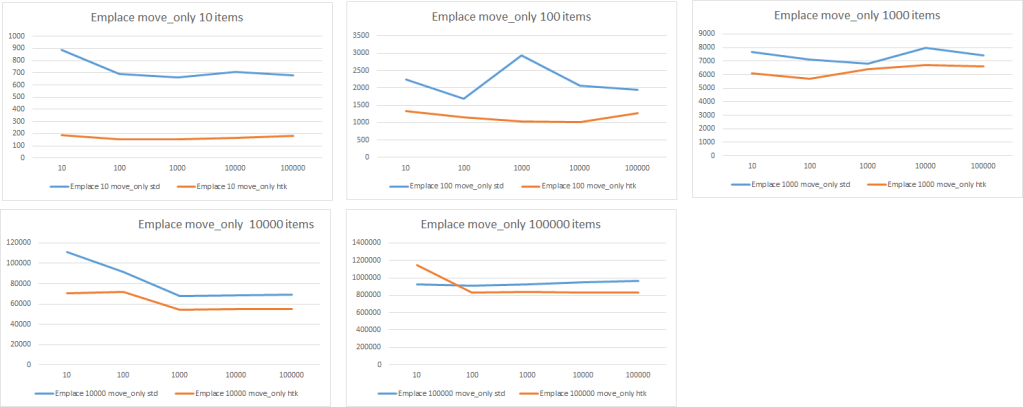
Here’s the graphed results of the different emplace measurements. On the x-axis, is the number of iterations the test was run, on the y-axis is the time in nanoseconds. The blue line represents the MSVC standard vector, and the orange line is the htk vector. Well — no surprise here, htk wins. No need to look any closer at those results.
Just kidding. Put your pitch-forks away. I don’t actually think that the htk vector is more performant than the MSVC vector. There’s perfectly logical explanations to why it is coming in faster than the STL vector. One plausible answer would be that the numbers are just way off, I’ve never claimed to be a mathematician or statistician. The code could be wrong, there’s a possibility that I’m timing more than I’d like to be timing. However, given that the code is identical for both cases, it should be consistent. I will say however, that there is large variance in the data.
| name | iterations | total | mean | median | min | max | s-dev |
| vector<int> emplace 10 | 10 | 61200 | 5160 | 2500 | 1700 | 27300 | 7515.344 |
| vector<int> emplace 10 | 100 | 268200 | 2162 | 2100 | 1500 | 6000 | 530.2405 |
| vector<int> emplace 10 | 1000 | 2993100 | 2391.5 | 2200 | 1600 | 20900 | 1051.978 |
| vector<int> emplace 10 | 10000 | 24818400 | 2022.05 | 1900 | 1000 | 1900700 | 19016.71 |
| vector<int> emplace 10 | 100000 | 121941400 | 997.8218 | 800 | 600 | 375300 | 2574.748 |
With such a large standard deviation, it means are data is pretty widely spread, and using Bryce’s check to determine if the values are normally distributed. Hardly any of the tests were seemingly normal. That being said, I ran the measurements multiple times, and saw similar results so, let’s go with it being somewhat correct.
We can start to reason about why the htk vector might be faster than the standard vector? Well — truth be told, there was one test that I knew htk would have the upper-hand. The emplace 10 items test. Well — if you recall when we implemented our vector, the initialization of the vector allocated 10 slots. This means, that we started with enough room for 10 elements. The standard vector had to allocate this initial memory, so it was pretty safe to say we’d win there.
In two of the cases emplace 1000 and 10000, we didn’t actually win. If you look at the 100000 iteration trials for both tests, the timing was almost identical. So likely, at best for two of the cases we’re equal, which makes sense. To illustrate this further we’ll take the 100000 iteration trials, for each test 10 items, 100, 1000, 10000, 100000 items and graph that.

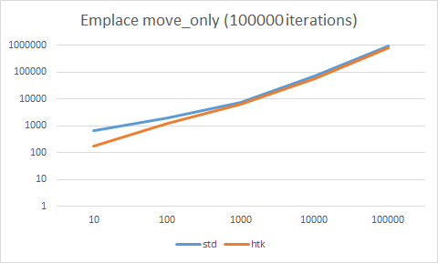
As we can see, the two are almost identical. Since our trial size is growing by a factor of 10 per test, it makes sense to plot the time on a logarithmic scale.
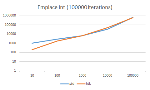
This graph, shows pretty clearly, almost exactly what we expected. In the test with 10 elements, the htk vector is superior because it isn’t doing any allocations. The 100 element makes sense it would be slightly faster, because we saved the time from the first 10 allocation. After that, it stops mattering. The two are pretty much neck and neck. Another reason I suspect as to why the htk vector might have a slight upper hand, for the move_only object, is that it’s much less safe. The htk vector probably doesn’t even offer a basic exception guarantee, whereas the stl vector offers a strong guarantee, whereby if an exception is thrown while the collection is growing, it will effectively roll back to the state before trying to grow. With the htk vector, well, it doesn’t do that. It at least tries to clean up for a basic guarantee, but I didn’t really pay attention to ensuring it, so there could be cases where it does not offer that.
Okay — so now for the embarrassment I think we were all expecting.

Overall — I’d say this is a blow out, the std vector is about 5x faster in all cases than our htk vector. So then we ask ourselves, why? Well, the answer lies back with what we did for emplace, and what we didn’t do for insert. Well, kind of. With the insert, when we need to grow if the original items, and they’re trivial items, we can just use memmove to very quickly move the contiguous data from one area of memory to another. Keeping in mind, this is trivial data which is what allows us to just copy the bytes. This definitely optimized our growth code for trivial types. However, when we implemented insert we used this code:
move_items(data_.first, data_.first + offset, next.first, copy_type{});
auto dest = first + offset;
while (start != fin)
    allocator_.construct(*(dest++), *(start++));
move_items(data_.first + offset, data_.last, dest, copy_type{});
You can see that we use our tag dispatch optimized function to move the items within our vector around, but when we’re inserting our new elements, we just construct them one by one. Instead of just moving them (read: memmove) into the newly allocated space. Now, you might be asking “how much slower could that actually be?” Well, in this case, it turns out to be roughly 5x slower, in fact. So we can change the code to something along the lines of…
move_items(data_.first, data_.first + offset, next.first, copy_type{});
auto dest = first + offset;
move_items(start.ptr(), fin.ptr(), dest, copy_type{});
move_items(data_.first + offset, data_.last, dest, copy_type{});
If you recall, when we wrote move_items, we took advantage of tag dispatching, to determine which function to use. The specific function that will get chosen will be the function that uses memmove.
void move_items(pointer first, pointer last, pointer &dest, memcpy_items_tag)
{
     memmove(dest, first, (last - first) * sizeof(T));
}
After changing the code, I re-ran the insert tests, and the results (unsurprisingly) looked like this.
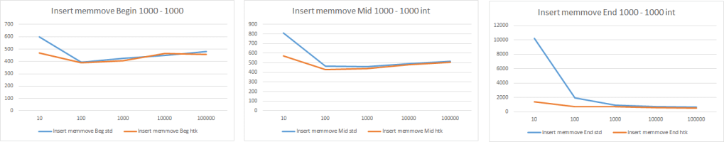
You can see now, they’re both really fast, given that they’s within 200ns of each other. I’d say that they’re pretty much identical. The only justification I can make for the slight difference, is again the safety factor. We really don’t care about any exception guarantees, which for fun is okay, but don’t try it at work.
Okay — I’ll address it. I know it’s burning for some of you. That code I wrote above, doesn’t actually work. I mean — it works, for the test I had written, but not much else.
move_items(start.ptr(), fin.ptr(), dest, copy_type{});
This line here, has this weird .ptr() call on both the iterators. I can explain. Basically, for move_items, which is akin to the MSVC _Umove function. However, the MSVC functions work on iterators, and ours just so happens to work on pointers, from the legacy code we wrote in the first article. What does that mean? Well, it means that we directly pass the input to our move_items call into memmove. This was perfect at that time, because we had full access to the pointers. Meaning our iterator was a pointer. But now, now we’re working with iterators that aren’t pointers. Just so we’re on the same page, a pointer is an iterator, but an iterator is not a pointer. There is a level of indirection there, that allows iterators to work the way they do over pointers, but it means we can’t feed the iterator directly into the memmove function without the compiler yelling. But you just said that MSVC uses iterators in their function…. They do, but first they go through the process of undressing their iterators. No — wait, that’s not right. Unwrapping, their iterators. It’s basically the processes of removing the iterator facade so that we can in this case see the underlying pointer. But why didn’t you do that, Peter? Well — if I’m honest, as much as I love rabbit holes, and going down them to come out the other side. I’m probably almost as tired of working on this vector, as you readers are reading about it. It’s also another exercise in traits, and meta programming that I didn’t want to spend the time on. My bad. 🙂
I had a better use of that time. I’m going to try and keep my promise that I made in the beginning, and in the middle, and now as we approach the end. I still have not kept. I have not really talked at all about implementing OR timing an algorithm.
So — the other day, I was listening, or watching, I think listening to a CppCast Podcast, and Sean Parent was the guest. He was talking about how at Adobe one of the technical questions is that you have to implement a binary search, and then prove it. I thought, challenge accepted. Not that I’ll be applying at Adobe any time soon, but it’s a worth while exercise. Especially when it’s not for all the marbles, like a job at Adobe.
template <typename IteratorT, typename ValueT>
bool binary_search(IteratorT begin, IteratorT end, const ValueT &v)
{
    const int mid = (end - begin) / 2;
    if (mid == 0)
        return *begin == v ? true : ( *(end-1) == v ? true  : false);
    const auto midval = *(begin + mid);
    if (midval == v)
        return true;
    if (v < midval)
        return htk::binary_search(begin, begin+mid, v);
    else
       return htk::binary_search(begin + mid, end, v);
}
Okay — I did it. It’s a recursive binary search function. I know what you’re thinking, eww recursion. That’s just how I think about it. So the the next part, is to prove it by induction. Dun. Dun. Dun. Now, Sean mentioned that he had an individual provide 30 pages of documentation for the binary search. I’ll attempt to do one better…. 31 pages! Just kidding. I can barely muster 5000 words into a coherent blog post, let alone a 31 page proof.
Here it goes. Given that we have a ascending sorted collection. Our base case is a collection of 2 items, where the midpoint(end-begin)/2 will be equal to 0, when this is the case the value we’re looking for must be one of those two values, or does not exist. In the case where the collection is larger than 2, our midpoint is not equal to 0. There are three cases, if the value of our midpoint is equal to our value, it exists in our collection. If it is not equal, and the search value is less than the value of our midpoint then it can only exist in the bottom half of the collection. If the value is greater than the midpoint value, then it can only exist in the top half of the collection.
Well, it’s not much, and it’s hardly a mathematical proof, but it’s my best try. I think it illustrates the point of binary search as divide and conquer.
To close off this post, my plan was to illustrate the magic of the binary_search over the plain old linear search. However, like always, color me surprised. I went off an used the chronograph library to time the different search functions. I wanted to test std::find, std::binary_search, and htk::binary_search (recursive) to see how they fair across a vector of integers. So the test was as follows.
- Generate a random vector of size 10, 100, 1000, 10000, with values between 1-100
- Generate a random search value between 1 – 100
- Test 10, 100, 1000, 10000, 100000 times, each search function
As simple as this seems, it wasn’t as straightforward as I would have thought. My first hurdle was that my “random” generator function, wasn’t really random. The initial code looked like this.
template <typename T, typename VectorT>
VectorT random_numeric_vector(size_t size, T min = std::numeric_limits<T>::min(), T max = std::numeric_limits<T>::max())
{
    VectorT v;
    std::default_random_engine generator;
    std::uniform_int_distribution<T> distribution(min, max);

    for (size_t i = 0; i < size; ++i)
    {
        v.emplace_back(distribution(generator));
    }
    return v;
}

size_t next_random(size_t min, size_t max)
{
    std::default_random_engine generator;
    std::uniform_int_distribution<size_t> distribution(min, max);
    return distribution(generator);
}
A simple test case looked like this.
benchmark(s, "std::binary_search vector<int>(10)", [](session_run &r) {
    auto v = random_numeric_vector<int, std::vector<int>>(10, 1, 100);
    std::sort(v.begin(), v.end());
    auto value = next_random(1, 100);
    measure(r, [&v, &value]() {
        std::binary_search(v.begin(), v.end(), value);
    });
});
The result I was seeing, across the two searches were very, very strange. The linear search sat somewhere in the realm of 100ns, for every collection size. The binary search, was slower, somewhere in the range of ~150ns, and slightly higher for the larger collection, not much though. So I thought, what the heck? I chalked it up to something to do with optimization. So, I chased down some code to tell the optimizer to eff off, and I ran it again. Same result. Over an over. In hindsight, I probably should’ve checked the documentation, or been smarter. It took me putting a debugger on to look, and see. Every time I would generate a new “random” vector, it was the same random values. As well, each time I would generate a “new” random search value, it just so happened to be equal to the first element in the collection. Thus, my pseudo random number generator, using a new default_random_engine per call, was giving me the exact same set of random values. Which just so happened to make each random search value, not so random. In fact, it was the best case for a linear search, making it return in every iteration, and every vector size, immediately.
After all that. I fixed the issue by hoisting and reusing the default_random_engine, so I was getting a set of random values. So then back to timing it. After I ensured the values were random, and the test was definitely executing the code I wanted. I had hoped to see the results we talked about earlier. You know, where the linear search time grew exponentially as the collection grew exponentially. Then where the binary search time grew, and then as the collection got larger and larger, the time to search leveled off. A logarithmic graph.

Then this happened. What. The. Fox. Said? The one I least expected, std::find is fastest, almost in all cases. They’re basically equivalent up until a million items, where I would’ve expected the binary_search to prevail. The linear search, performing like that is very strange. Not only does it out perform both the linear searches (loop style & recursive), it also doesn’t require the input to be sorted, which on average took almost 33 ms to sort the 1 000 000 000 int vector. That is quite a bit of overhead to pay, just to be outperformed. What gives? This isn’t what my CompSci professor told me, they couldn’t have been lying could they? Obviously, it makes logical sense that a linear search, whereby you could potentially have to iterate all elements, would take more time than one where continually break the search in half. So, my professor wasn’t lying, and this result is just very counter intuitive. We can make a bet that std::find isn’t doing what we think. It just can’t be. Let’s prove that.
We are assuming it’s iterating the collection and checking, something like this.
template <typename IteratorT, typename ValueT>
bool linear_search(IteratorT begin, IteratorT end, const ValueT &v)
{
    for (; begin != end; ++begin)
    {
        if (*begin == v)
            return true;
    }
    return false;
}
Update 06.16.2020: After posting this story to reddit, it was pointed out by /u/staletic that std::find is not optimized by memchr. In fact, after I stepped through with the debugger, it was in fact, not doing this. I’m wondering if it’s just the sheer act of unwrapping the pointers to raw pointers that is making it that much faster. I’m going to run a test and see.
I ran the results of that test, and voila!
| Size | 10 | 100 | 1000 | 10000 | 100000 | 1000000 |
| std::find | 249.341 | 195.602 | 205.812 | 171.916 | 266.472 | 513.4 |
| std::binary_search | 96.202 | 129.227 | 163.582 | 206.146 | 409.685 | 1321.187 |
| htk::binary_search | 108.538 | 143.235 | 161.051 | 196.494 | 504.58 | 1114.834 |
| htk::linear_search | 85.808 | 126.395 | 421.989 | 3577.376 | 34773.36 | 391704.3 |
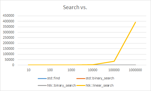
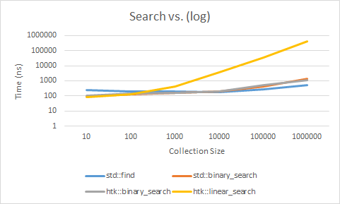
So, the first graph looks a lot more like we would’ve assumed it to look, the linear search grows exponentially as our collection grows exponentially. It also gets trounced by even the recursive binary_search. Which even makes the cost of sorting the collection totally worth it. That said, if you’re able to not pay the sort cost, by maybe, maintaining sort order on insert. You have a very quick search on your hands.
So what gives with std::find, well the truth is in the details. It looks like for types that aren’t trivial types, it does a typical linear search, in the style we implemented. But, when it comes to trivial types, it uses a different mechanism. It uses a call to memchr, a C-api call that will find the pointer to a matching value in a set of data. Though I’m not sure how it’s implemented, I can tell you, it’s very quick. Meaning that if you have a collection of trivial types, it looks to be in your best interest to favor std::find for searching the collection, and not worry about having to sort the collection.
Alright — I think I kept my promise. That was long winded, but a surprisingly interesting journey. We scratched the surface of micro-benchmarking, by understanding how to apply it to the work a vector does. As well, we took a stab at implementing (and proving) a binary_search algorithm. Then, we got to see it in action, and how it performed (or should I say got out performed) against std::find and std::binary_search, then we saw how a true linear search really compares to a binary search, when they’re playing the same game. Overall, this was a very interesting walk down vector trail. I hope you enjoyed the read, and look forward to seeing you next time!
Until then, stay healthy, and Happy Coding!
PL
A sudden bold and unexpected question doth many times surprise a man and lay him open.
Francis Bacon
References
https://www.youtube.com/watch?v=zWxSZcpeS8Q&feature=youtu.be
https://www.youtube.com/watch?v=nXaxk27zwlk&feature=youtu.be&t=2441
https://www.bfilipek.com/2016/01/micro-benchmarking-libraries-for-c.html
https://github.com/google/benchmark/blob/c078337494086f9372a46b4ed31a3ae7b3f1a6a2/include/benchmark/benchmark.h
https://github.com/rmartinho/nonius

Leave a comment